rick-gilmore.com - Thanks, Mike

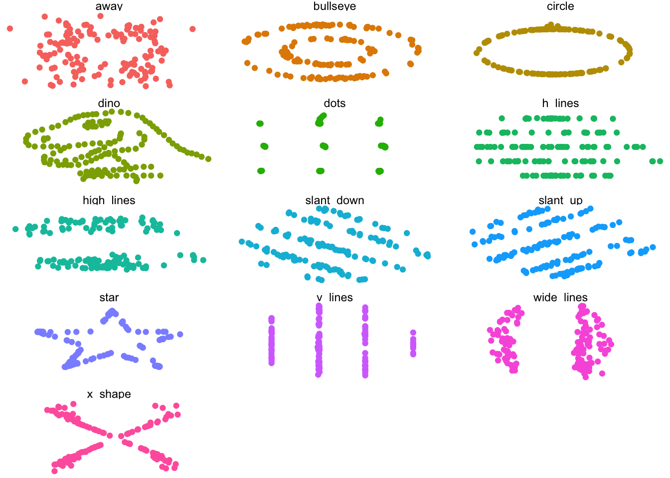
One stats class was required in my grad program, and Mike Meyer was my professor. The class was in S-plus, the closed source inspiration for R. And Mike regularly exhorted us (in his inimitable Australian accent), “Plot your data!”

Mike’s encouragment to use S-plus made it easier for me to adopt R when it appeared on the scene a few years later. Or at least I had fewer habits to change. And, Mike’s advice about plotting your data first always made sense to me. If you can’t see a pattern in the plots, how can you believe the inferential statistics?

In that spirit, mostly so that I can find it again, is an outstanding demonstration of that truth, the datasauRus package, based on Anscombe’s quartet (Anscombe 1973), which is also available as the anscombe package.

library("ggplot2")
library("datasauRus")
ggplot(datasaurus_dozen, aes(x = x, y = y, colour = dataset))+
  geom_point() +
  theme_void() +
  theme(legend.position = "none")+
  facet_wrap(~dataset, ncol = 3)

These all have roughly the same summary statistics.

if(requireNamespace("dplyr")){
  suppressPackageStartupMessages(library(dplyr))
  datasaurus_dozen %>% 
    group_by(dataset) %>% 
    summarize(
      mean_x    = mean(x),
      mean_y    = mean(y),
      std_dev_x = sd(x),
      std_dev_y = sd(y),
      corr_x_y  = cor(x, y)
    )
}

# A tibble: 13 × 6
   dataset    mean_x mean_y std_dev_x std_dev_y corr_x_y
   <chr>       <dbl>  <dbl>     <dbl>     <dbl>    <dbl>
 1 away         54.3   47.8      16.8      26.9  -0.0641
 2 bullseye     54.3   47.8      16.8      26.9  -0.0686
 3 circle       54.3   47.8      16.8      26.9  -0.0683
 4 dino         54.3   47.8      16.8      26.9  -0.0645
 5 dots         54.3   47.8      16.8      26.9  -0.0603
 6 h_lines      54.3   47.8      16.8      26.9  -0.0617
 7 high_lines   54.3   47.8      16.8      26.9  -0.0685
 8 slant_down   54.3   47.8      16.8      26.9  -0.0690
 9 slant_up     54.3   47.8      16.8      26.9  -0.0686
10 star         54.3   47.8      16.8      26.9  -0.0630
11 v_lines      54.3   47.8      16.8      26.9  -0.0694
12 wide_lines   54.3   47.8      16.8      26.9  -0.0666
13 x_shape      54.3   47.8      16.8      26.9  -0.0656

And here are the originals from (Anscombe 1973):

with(anscombe, plot(x1, y1))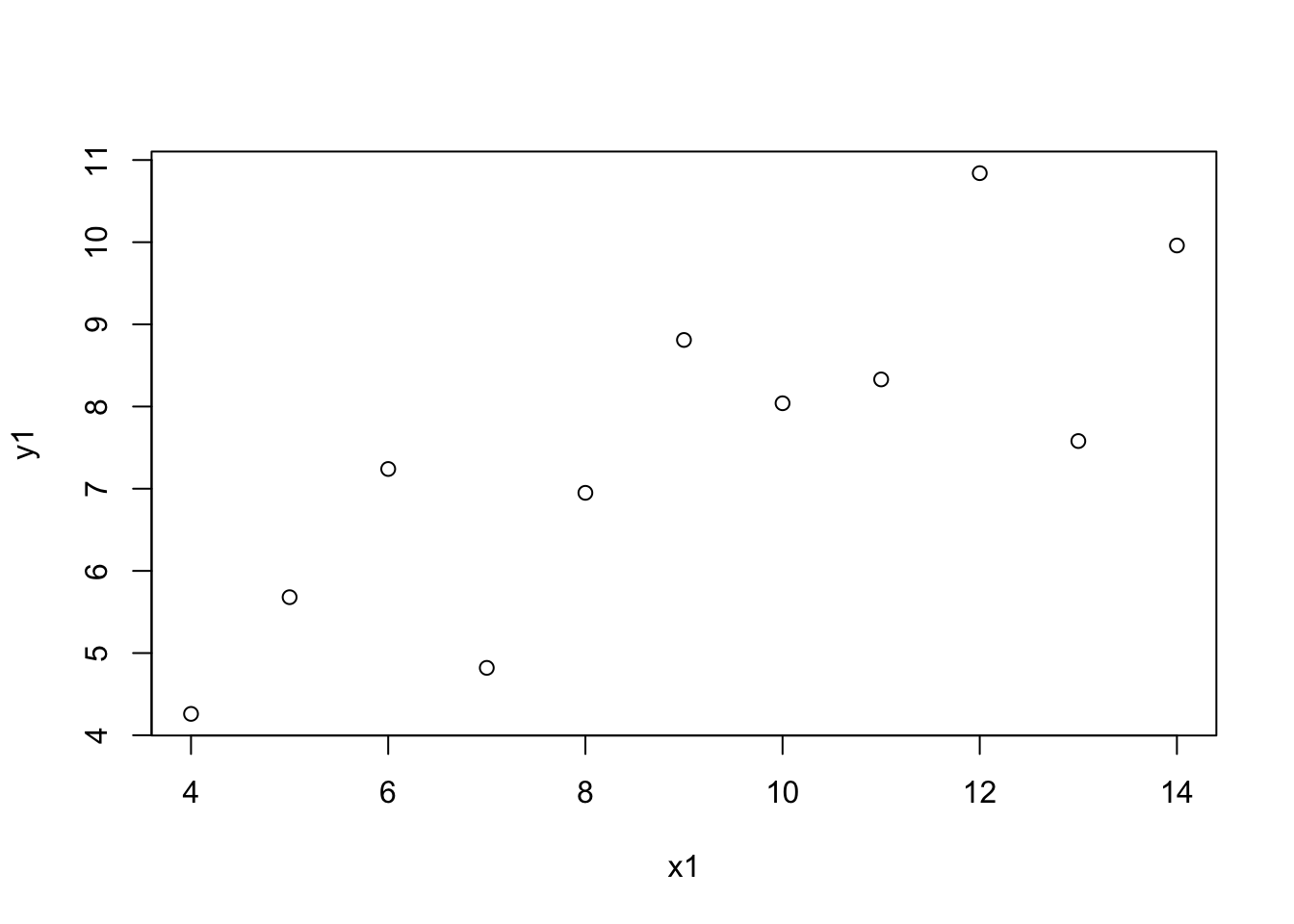

with(anscombe, plot(x2, y2))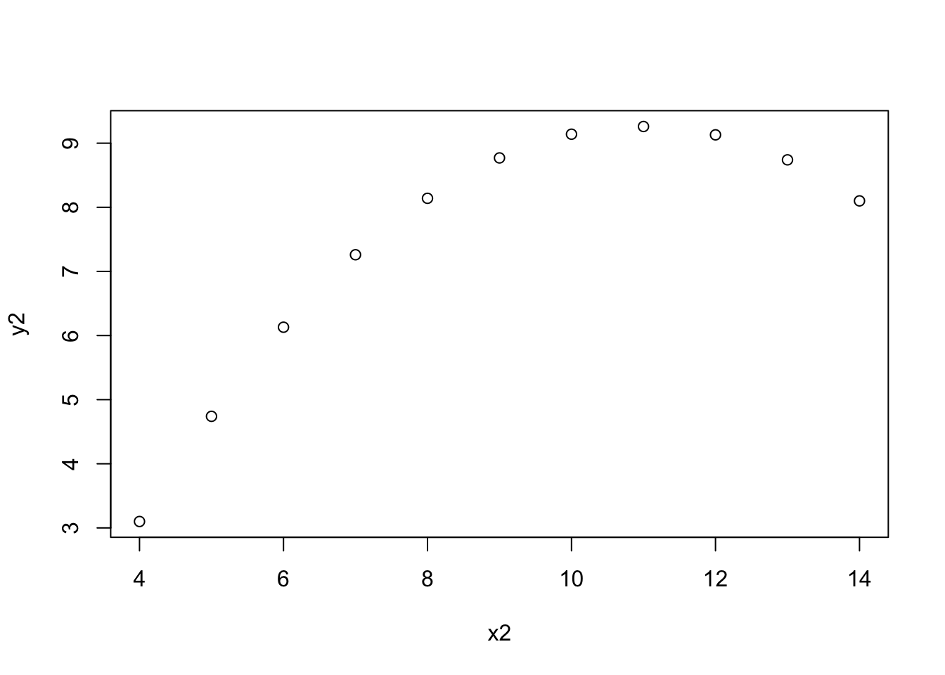

with(anscombe, plot(x3, y3))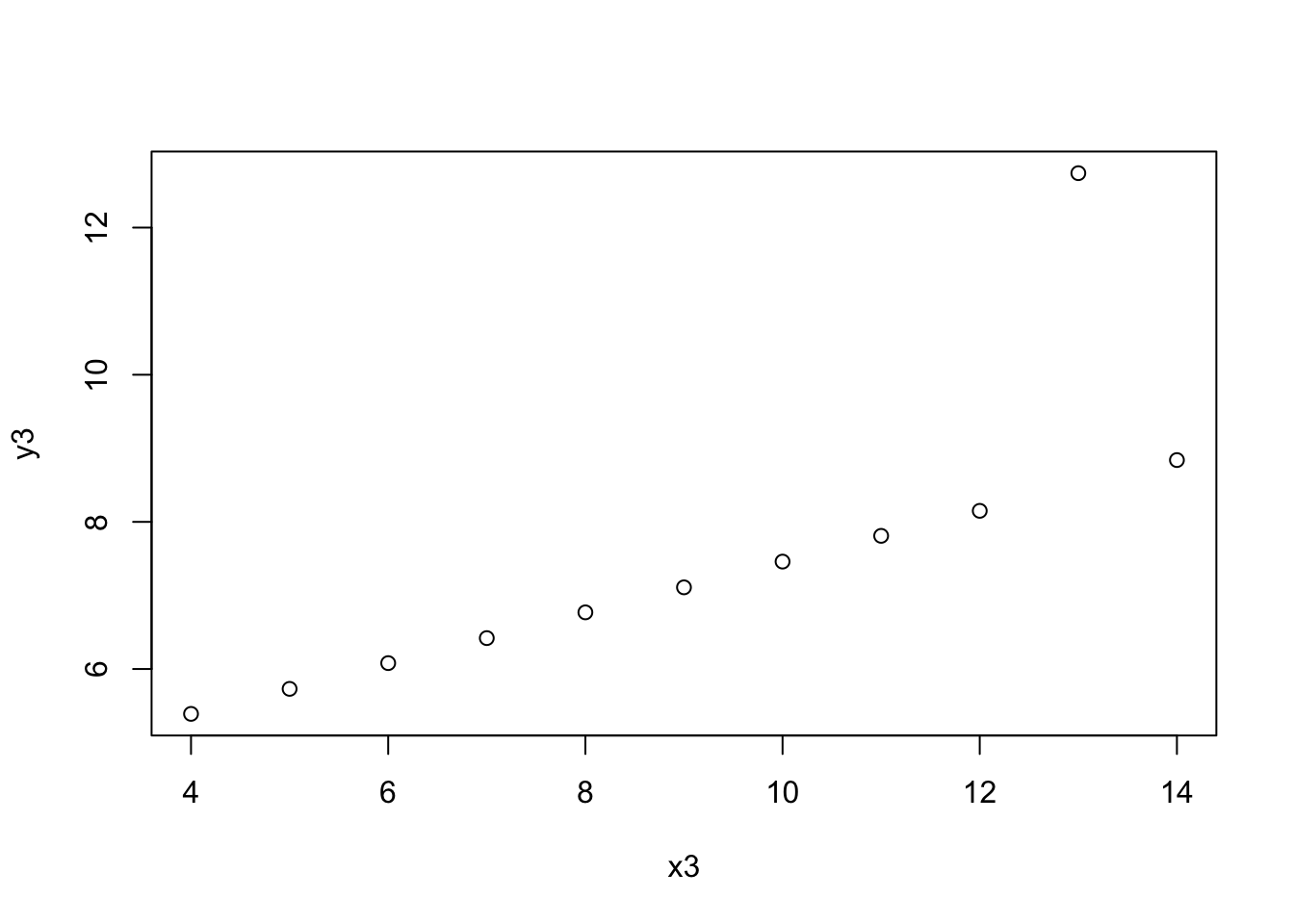

with(anscombe, plot(x4, y4))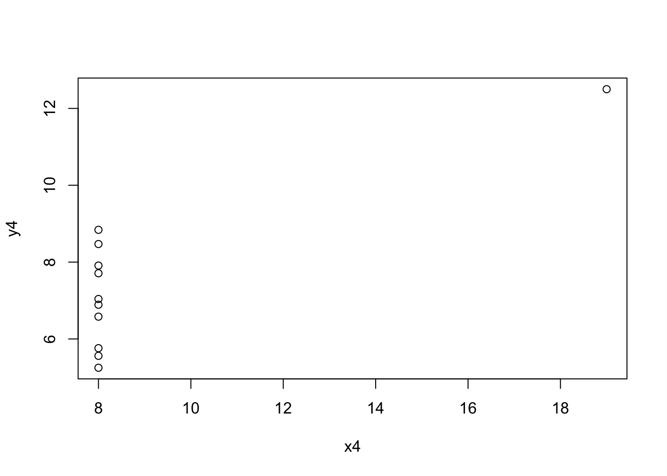

Thanks for giving me such a great start in statistics, Mike! I’m sure if the Datasaurus had been around then, you’d have been a fan.

References

Anscombe, F. J. 1973. “Graphs in Statistical Analysis.” American Statistician 27 (1). https://doi.org/10.1080/00031305.1973.10478966.